A Hybrid Search Case Study: Widely Applicable Techniques for Ranking Better Results

Most search implementations in production fall into one of two camps: pure vector similarity that returns plausible but wrong results, or keyword search that misses anything not phrased exactly right. Neither is good enough when the stakes are real — when a bad match means a wasted introduction, a missed collaboration, or a researcher paired with the wrong domain expert.

This post uses a hybrid expert-matching system over a corpus of ~200,000 profiles as a concrete case study. If you’re trying to decide which search techniques you actually need, the useful question is not “should we add AI?” but rather “what kind of ranking mistake are we trying to fix?”

A useful mental model is this: the obvious buzzword match is often what a user expects to see first, but not always the most helpful recommendation. A good system should be able to say, in effect, “Yes, here is the straightforward person you probably had in mind — and here are the two or three people who can actually get you further.” The hard part is choosing the techniques that produce that behavior intentionally rather than by accident.

Questions That Shape the Ranking System

Before choosing techniques, it helps to be explicit about the problem you’re solving. Different search systems fail for different reasons, and those failures should determine what gets built.

Question that shapes the system	Engineering implication
What does a good match look like?	Ranking objectives and evaluation examples
What kinds of results are plausibly relevant but still feel misaligned?	Soft penalties, diversity, and explanation surfaces
What terms are essential vs. adjacent?	FTS query construction, concept weighting, structured boosts
What should be discouraged but not excluded?	Demotions rather than hard filters
What would make a user trust the result?	Diagnostics, traceability, and result explanations

The point is not to force a formal handoff between “business” and “engineering.” The point is to make sure the ranking system is answering the right questions. A good hybrid system is usually the result of translating these domain questions into explicit retrieval and ranking signals.

Choosing Techniques by Failure Mode

Once the failure modes are clear, the next question is which techniques actually address them. The cleanest way to think about this is not as a tree but as a mapping from ranking pathology to intervention:

If the search fails because…	Add this technique	Why it helps
The query and the right answer use different language	Semantic retrieval (vector search)	Captures conceptual similarity beyond exact wording
Exact credentials, acronyms, or procedures matter	Lexical retrieval (FTS)	Preserves precision on terms that should not be semantically blurred
The raw query is vague, underspecified, or constraint-heavy	Query analysis	Extracts intent, concepts, and discouraged modalities before retrieval
Some signals should count more than others	Structured boosts and penalties	Encodes domain judgment directly into ranking
The top candidates are plausible but poorly ordered	Cross-encoder reranking	Adds expensive precision after cheap retrieval narrows the field
The top results are individually relevant but too similar to each other	MMR diversification	Trades a little rank optimality for variety across the final set
People do not trust the output	Diagnostics and explanation surfaces	Exposes why a result ranked highly and which signals mattered

This is the core design principle: a useful hybrid system is not just “semantic + keyword.” It is a deliberate composition of stages, where each technique is introduced to correct a specific class of failure.

The Problem With Naive Vector Search

Vector search feels magical in demos. Embed your corpus, embed your query, find the nearest neighbors. Ship it.

Then you hit production and discover:

Failure Mode	What Happens	Why
Semantic drift	“bone density expert” returns MRI technicians	Vector similarity conflates domain adjacency with expertise match
Profile quality blindness	Empty profiles rank as high as rich ones	Cosine distance doesn’t know a profile has no content
Result homogeneity	Top 5 results are from the same subspecialty	Nearest neighbors cluster in vector space
Keyword gaps	Exact credential/procedure matches get buried	Embedding models compress precise terms into vague neighborhoods

If you’ve shipped vector search and noticed users not trusting the results, these are probably why.

The Problem With Naive Keyword Search

Full-text search has the opposite failure mode. It’s precise but brittle:

• Synonym blindness: “heart failure” misses “cardiac insufficiency”
• No semantic understanding: can’t match “someone who studies aging bones” to an osteoporosis researcher
• Exact-match bias: rewards profiles stuffed with keywords over genuinely relevant experts

Neither approach alone is sufficient. The question is how to combine them without the combination being worse than either part.

A Five-Phase Ranking Pipeline

Here’s the architecture that emerged. It can be read as a technical stack, but it is more useful to read it as a sequence of design questions: what is the user really asking, what evidence should count, how do you combine unlike signals, how do you avoid redundant results, and how do you explain what happened when someone challenges the output?

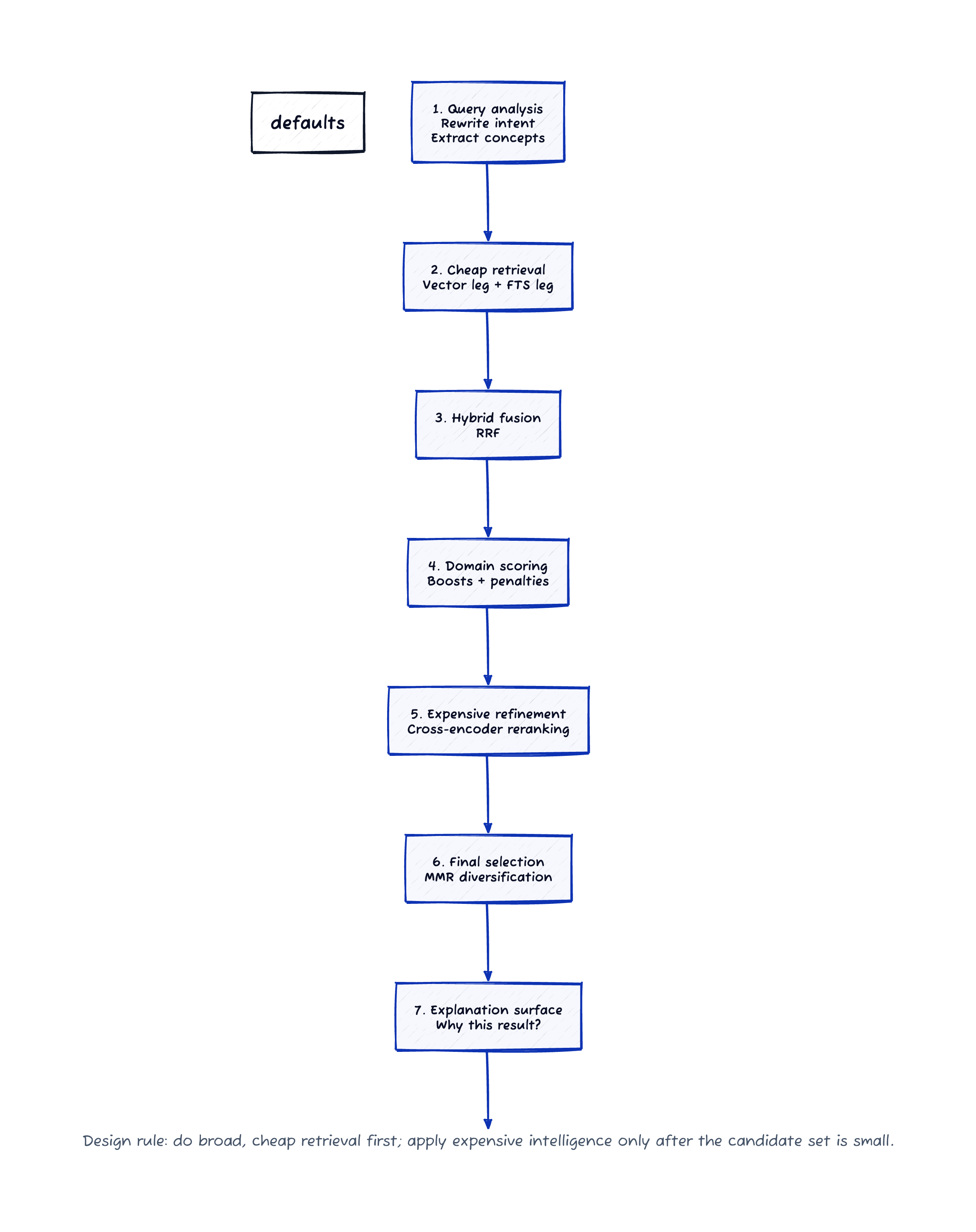
Click the diagram to view it full size.

Phase 0: LLM Query Analysis

Before any retrieval happens, the raw query goes through a lightweight LLM call (using a small, fast model at temperature 0) to produce a structured search plan:

User query: "bone density assessment without ionizing radiation"

Parsed output:
  expert_intent_query: "bone mineral density skeletal health aging"
  expert_concepts: ["bone mineral density", "skeletal health"]
  supporting_domain_terms: ["osteoporosis", "DXA alternative"]
  discouraged_modalities: ["ionizing radiation", "CT", "DXA"]

The critical design decision here: The query analyzer preserves expert intent, not solution intent. It does not rewrite “bone density without radiation” into “ultrasound expert” — that would be the system guessing the solution. Instead, it searches for bone density experts and applies soft penalties to those primarily associated with the discouraged modalities.

This distinction matters more than anything else in the query understanding layer. Systems that pivot on constraints instead of expert intent often return completely wrong results — searching for the alternative technology instead of the domain expert.

Graceful degradation: If the LLM call fails, the system falls back to embedding the raw query directly. No hard dependency on the query analyzer.

Sidebar: Guardrails vs Penalties

When a user says “I don’t want X,” the instinct is to build a hard filter. Don’t. Hard filters in search are brittle. If you filter out all experts who mention “DXA” (the standard bone density scan), you might filter out the exact expert who just published a paper on alternatives to DXA.

Instead, treat these constraints as soft penalties. The expert still enters the candidate pool, but their score is reduced. This is a recurring pattern in robust search systems: prefer soft signals (boosts and penalties) over hard gates (filters) unless the constraint is absolute (like location or availability).

Phase 1: Reciprocal Rank Fusion (RRF)

In a hybrid system, you run multiple independent retrieval streams—often called “legs”—and combine their results. Here, we build and fuse two lists:

The Vector Leg: Embed the optimized query, find each expert’s best-matching embedding chunk by cosine distance, deduplicate per expert, and rank by semantic similarity.

The Full-Text Search (FTS) Leg: Build a phrase-aware tsquery from the parsed concepts and domain terms. Words within each concept are AND’d; concepts are OR’d. Prefix matching (term:*) handles inflectional variants. Rank by ts_rank_cd (a standard keyword density metric).

Fusion: Combining these is tricky because vector similarity scores (e.g., 0.85) and keyword density scores (e.g., 2.4) aren’t mathematically comparable. Enter Reciprocal Rank Fusion (RRF). Instead of looking at the raw scores, RRF only looks at the rank a candidate achieved in each list:

RRF_score = 1/(K + vec_rank) + 1/(K + fts_rank)

K=60 is the standard damping constant. If an expert is rank 1 in the vector leg, they get 1/61 points. If they are rank 2 in FTS, they get an additional 1/62 points.

Experts absent from one leg receive a soft penalty rank (not exclusion) — this is important because an expert who matches semantically but not lexically should still appear, just with a lower combined score.

Why RRF over learned fusion? RRF is parameter-free (just K), doesn’t require training data, and is remarkably robust. It prevents one retrieval method from wildly overpowering the other. For expert matching where you don’t have historical click-through data to train a fusion model, RRF is the right default.

Phase 2: Structured Field Boosting + Penalties

Vectors and keywords capture what someone talks about. They don’t capture the nature of the expertise. After fusion, domain-specific signals adjust scores to account for where and how the expertise appears.

Structured field boost: Expert metadata fields (research areas, departments, procedures, credentials) are checked against parsed query concepts. Matches are weighted by specificity:

Match Location	Weight
Research areas / interests	+3 per concept
Departments / procedures	+2 per concept
Profile URLs / bio text	+1 per concept

This matters because an expert whose research areas include “bone mineral density” is a stronger match than one who merely mentions it in a long bio.

Discouraged modality penalty: As mentioned in the sidebar above, experts primarily associated with approaches the user wants to avoid receive a soft score reduction. This is demotion, not exclusion.

Evidence quality penalty: Sparse profiles — those with just a name and title, no bio, no research areas — are penalized. An expert you know nothing about is not a confident recommendation. If a profile is too sparse (e.g., just a name and title), the system can even gate them from the expensive reranking phase to save compute.

Phase 3: Cross-Encoder Reranking

The top candidates are reranked using a cross-encoder (in this case, Google’s Vertex AI Ranking API).

To understand why this helps, you have to understand the difference between bi-encoders and cross-encoders. In Phase 1, we used a bi-encoder: the query and the document were embedded completely independently, and we just measured the geometric distance between their vectors. It’s incredibly fast, but semantically coarse.

A cross-encoder feeds the query and the document together into a transformer network. The model gets to see how the words in the query relate to the words in the document via attention mechanisms. It’s much more computationally expensive (you can only run it on dozens of documents, not thousands), but deeply accurate contextually.

Sidebar: The Reranking Trade-off

If cross-encoders are so much better, why not use them for everything? Because they don’t scale. You can’t pre-compute a cross-encoder score the way you can pre-compute a bi-encoder vector, because the cross-encoder score depends on the specific query. You have to run the neural network at query time for every candidate.

This is why search pipelines are funnels: Phase 1 (bi-encoder + FTS) is the cheap, wide net that finds the top 100. Phase 3 (cross-encoder) is the expensive microscope that perfectly sorts the top 10.

Three practical rules make reranking usable rather than magical:

1. Build query-aware payloads. Don’t just send the full profile. For each candidate, the system selects the best-matching bio excerpt (by term overlap with the query) and combines it with structured metadata. This gives the reranker focused signal.

2. Gate noise candidates. Profiles with thin content or vector-only matches (no lexical signal) produce poor reranker inputs. The system gates them out before reranking to prevent noise from diluting the reranker’s attention.

3. Detect low-variance reranker output. Sometimes the reranker returns nearly identical scores for all candidates — meaning it couldn’t differentiate them. When that happens (≤2 distinct scores in the top 10), the pipeline falls back to the pre-rerank order rather than letting the reranker randomly shuffle.

Phase 4: MMR Diversification

If your top five results are all identical clones of each other, your user didn’t get five choices; they got one choice, repeated. The final selection uses Maximal Marginal Relevance (MMR) to balance relevance against redundancy.

MMR is a greedy algorithm. It picks the most relevant result first. Then it looks at the remaining candidates and picks the one that offers the best mix of high relevance and high dissimilarity to what’s already been picked.

MMR scores the remaining candidates like this:

MMR_score = λ × relevance − (1−λ) × max_similarity_to_already_selected

• relevance: How good is this candidate for the query?
• max_similarity: How similar is this candidate to the experts we’ve already put in the final list?
• λ (lambda): A tuning knob (0 to 1) that controls how much you care about relevance vs. diversity.

The key insight: composite relevance is computed by blending scores from all prior phases — not just the reranker output. This preserves information from the RRF and structured boost phases into the diversification step, rather than treating the reranker as the sole arbiter of relevance.

With λ=0.8 (heavily relevance-weighted, but intolerant of exact duplicates), MMR ensures the top results span different subspecialties rather than clustering in one corner of the expert space.

Embedding Strategy: Not All Chunks Are Equal

The embedding layer deserves its own section because most tutorials treat it as “just call the embedding API.” In production, the decisions here cascade through everything downstream.

Separate structured metadata from narrative

Each expert has two kinds of content: structured fields (research areas, credentials, departments) and a narrative bio. The system embeds them as separate chunks. This prevents a long bio from diluting the precise structured signal, and it means vector search can match on either the structured or narrative dimension independently.

Sidebar: Why Chunking Matters

Embedding models compress text into a fixed-size vector (usually 768 or 1536 numbers). If you embed a 10-word sentence, the model captures that specific idea perfectly. If you embed a 10-page document, the model has to smash 10 pages of distinct ideas into the same 1536 numbers. The resulting vector becomes a blurry, generic average of everything.

To get precise search results, you have to break long documents into smaller “chunks” before embedding them. But how you break them up is the hard part.

Structure-aware bio chunking

Expert bios are not chunked by character count. The chunker respects document structure:

1. Split on paragraph boundaries first
2. If a paragraph is too large, split on sentence boundaries
3. If a sentence is too large, split on word boundaries
4. Hard-cut only as a last resort

This preserves semantic coherence within each chunk — a chunk boundary lands at a paragraph break if possible, not in the middle of a sentence about a specific research program.

Progressive chunk budgets

Rather than a fixed chunk size, the system uses progressive budgets: start with a generous budget (4,000 characters), and only tighten for texts that fail at the embedding model’s token limit. Most experts get fewer, larger, higher-quality chunks. Only the outliers (the experts with 10-page bios) get progressively smaller chunks.

This is materially better than a single conservative budget, which would fragment most bios unnecessarily, or a single aggressive budget, which would fail on outliers.

Symmetric vs. asymmetric embedding

For expert matching, the system uses symmetric SEMANTIC_SIMILARITY task type — the same profile for both indexing and querying. Both sides are “descriptions of expertise”: one from the expert’s perspective, one from the searcher’s perspective.

Why symmetric, not asymmetric? Google’s embedding API supports asymmetric task type pairs (RETRIEVAL_DOCUMENT / RETRIEVAL_QUERY) designed for cases where one side is a long document and the other is a short factual query. Expert search is different: both sides are descriptions of expertise — one from the innovator’s perspective (“I need someone who knows about bone density”) and one from the expert’s profile (research areas, bio, credentials). SEMANTIC_SIMILARITY is the correct task type for matching two descriptions against each other. The file content search pipeline uses the asymmetric pair because that relationship genuinely is document-vs-query.

Getting this wrong degrades retrieval quality silently — the vectors are in subtly different spaces and similarity scores become less meaningful.

Operational Lessons

Re-embedding 200k profiles without downtime

Our first implementation deleted all embeddings before rebuilding — meaning search was completely broken during re-embed runs. The fix was per-expert transactional replacement: load a page of experts, embed them, then in one transaction delete old rows and insert new rows for just those experts. Search stays live for all other experts throughout the rebuild.

Concurrency matters more than you think

Serial embedding of 200k profiles took 15+ hours. Adding bounded concurrent dispatch (8 in-flight embedding requests) brought it under 2 hours. The Vertex AI quota was never the bottleneck — our serial pipeline was.

Don’t retry deterministic errors

For Vertex specifically, INVALID_ARGUMENT is usually deterministic: if the request is invalid, retrying it just burns time.

Retry transient failures. Surface client errors immediately.

Tuning Parameters: Store Them in the Database

Five parameters control the ranking pipeline behavior. All of them are stored in the database with a short TTL cache, adjustable without code changes or deploys:

Parameter	Default	What it controls
mmr_lambda	0.8	Relevance vs. diversity balance
min_query_similarity	0.70	Cosine similarity floor — drop candidates below this
rerank_oversample	15	How many candidates enter reranking per result slot
rrf_k	60	RRF damping constant
candidate_multiplier	10	Oversample factor for each RRF leg

Being able to tune these in production without a deploy is essential. Search quality tuning is empirical — you adjust, observe, adjust again. Hardcoded constants mean every tuning cycle requires a deploy.

Build a Diagnostic Surface

This is the single most valuable investment in the entire system. A diagnostic endpoint exposes the full pipeline trace for any query:

• Query analysis output and timing
• Full RRF candidate list with per-candidate vector rank, FTS rank, and fused score
• Structured boost and penalty details per candidate
• Reranker input payloads, output scores, and gating reasons
• MMR selection trace with relevance scores and diversity decisions

When a user reports “the search returned the wrong expert,” operators can trace exactly why in seconds — which phase promoted or demoted that candidate, what the reranker saw, and why MMR selected or rejected them. Without this surface, search quality debugging is guesswork.

What’s Still Missing

No system is complete. Three next steps stand out:

• Offline evaluation framework: Labeled query/expert pairs with automated nDCG/recall@k measurement. Right now quality assessment is manual via the diagnostic surface.
• FTS concept weighting: The full-text leg treats all parsed terms equally. Primary expert concepts should be weighted more heavily than supporting domain terms.
• Adaptive chunk sizing: Using the embedding model’s own token counter to chunk precisely to the token budget, rather than using character-count heuristics.

Key Takeaways

1. Neither vector search nor keyword search is sufficient alone. RRF fusion with soft penalty ranks for missing signals is a robust default.
2. Query understanding matters more than retrieval sophistication. Preserving expert intent — not pivoting on constraints — is the highest-leverage design decision.
3. Reranking is powerful but fragile. Gate noise candidates out, build query-aware payloads, and detect low-variance output.
4. MMR diversification should blend all prior signals, not just the reranker’s opinion.
5. Build the diagnostic surface before you need it. You will need it. Search quality debugging without observability is guesswork.
6. Don’t retry deterministic errors. This sounds obvious, but getting it wrong can turn a 2-hour job into a 15-hour job.
7. Store tuning parameters in the database. Search quality tuning is empirical; deploy cycles are the enemy.